Un-Daming the Benthos

library(tidyverse)
library(readxl)
library(lme4)
library(lmerTest)
library(broom.mixed)
library(patchwork)
library(knitr)

Study Overview

“Slow drawdown, fast recovery: Stream macroinvertebrate communities improve quickly after large dam decommissioning” by Atristain et al. (2024) asked whether decommissioning the Enobieta Dam (42 m, northern Spain) restored downstream macroinvertebrate communities. They used a multiple Before-After/Control-Impact (mBACI) design, the ecological equivalent of difference-in-differences (DiD).

• Treatment: Reservoir drawdown (Dec 2018 - Nov 2019)
• Outcome: Macroinvertebrate community metrics (taxa richness, diversity, density, biomonitoring index)
• Design: Compare the change over time at impact sites (downstream of dam) vs. control sites (undammed tributaries)

In this post, we walk through a full replication of Atristain et al. (2024)’s mBACI analysis in R. We cover data loading and wrangling, exploratory visualization of the DiD structure, a linear mixed-effects model with annotated output and coefficient interpretation, an overall interaction test, model diagnostics, a robustness check across all four community metrics, and a critical evaluation of the causal assumptions and study limitations.

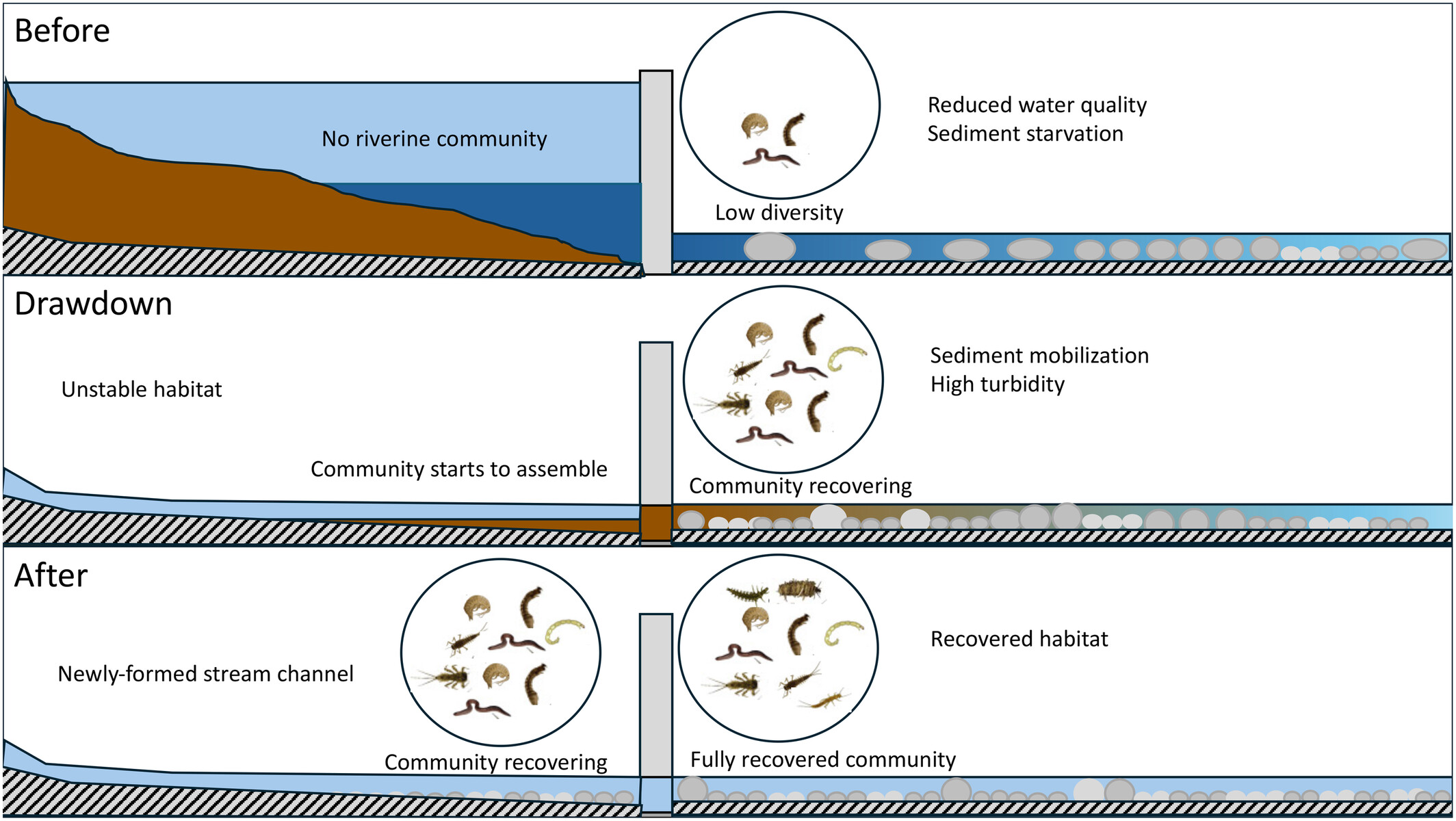
The figure below, reproduced from the paper’s supporting materials, illustrates how dam removal via slow drawdown transforms a degraded, low-diversity system into a fully recovered, biodiverse stream ecosystem. It conceptualizes the three stages (Before, Drawdown, and After) that form the basis of the statistical analysis.

NoteData Access

Data are from the Dryad Digital Repository. Download Atristainetal_JAE_Data.xlsx and place it in a data/ subfolder.

---

Data Loading & Description

invert_raw <- read_excel("data/Atristainetal_JAE_Data.xlsx",
                         sheet = "Invertebrates")

# two columns named "Site", rename for clarity
colnames(invert_raw)[1] <- "site_name"
colnames(invert_raw)[5] <- "site_code"

invert <- invert_raw |>
  select(site_name, Replicate, Period, Reach, site_code, S, `H´`, TD, IASPT) |>
  rename(richness = S, shannon = `H´`, density = TD) |>
  mutate(
    reach_type = case_when(
      Reach == "C" ~ "C",
      Reach == "R" ~ "R",
      TRUE ~ "I"
    ),
    period = factor(Period, levels = c("B", "D", "A"),
                    labels = c("Before", "Drawdown", "After")),
    reach_type = factor(reach_type, levels = c("C", "I", "R"))
  )

# filter to control + impact only (reservoir sites only sampled post-drawdown)
invert_baci <- invert |> filter(reach_type %in% c("C", "I"))

glimpse(invert_baci)

Rows: 120
Columns: 11
$ site_name  <chr> "Enobieta Up", "Enobieta Up", "Enobieta Up", "Enobieta Up",…
$ Replicate  <dbl> 1, 2, 3, 4, 5, 1, 2, 3, 4, 5, 1, 2, 3, 4, 5, 1, 2, 3, 4, 5,…
$ Period     <chr> "B", "B", "B", "B", "B", "B", "B", "B", "B", "B", "B", "B",…
$ Reach      <chr> "C", "C", "C", "C", "C", "I1", "I1", "I1", "I1", "I1", "C",…
$ site_code  <chr> "C1", "C1", "C1", "C1", "C1", "I1", "I1", "I1", "I1", "I1",…
$ richness   <dbl> 21, 23, 30, 30, 28, 6, 2, 4, 3, 3, 24, 20, 19, 11, 8, 10, 1…
$ shannon    <dbl> 2.7536694, 2.6475343, 2.6377758, 2.5200668, 2.6637126, 0.93…
$ density    <dbl> 2355.55556, 4277.77778, 2655.55556, 3277.77778, 1700.00000,…
$ IASPT      <dbl> 6.500000, 6.434783, 6.607143, 6.777778, 6.571429, 3.833333,…
$ reach_type <fct> C, C, C, C, C, I, I, I, I, I, C, C, C, C, C, I, I, I, I, I,…
$ period     <fct> Before, Before, Before, Before, Before, Before, Before, Bef…

Category	Description
Unit of observation	Five random samples collected with a Surber net (a standardized benthic invertebrate sampler covering 0.09 m²) from one site on one sampling occasion
Outcome variables	richness (S, taxa richness); shannon (H’, Shannon-Wiener diversity); density (TD, total invertebrate density); IASPT (Iberian Average Score Per Taxon, a pollution tolerance index)
Treatment	reach_type: Impact (I1-I4, downstream of dam) vs. Control (C1-C4, undammed tributaries + upstream)
Time	period: Before (Nov 2017), Drawdown (Oct 2019), After (Nov 2020)
Cleaning decisions	Reservoir sites (R) excluded, only sampled in the After period, so not usable for the before-after comparison
Sample size	120 samples total, 5 Surber net replicates x 4 sites per group x 3 periods; Artikutza protected catchment, northern Spain (2017-2020)

The four community metrics capture different but complementary dimensions of invertebrate recovery. Taxa richness (S) counts the number of distinct taxa present and is the most direct measure of biodiversity. Shannon diversity (H’) weights taxa by their relative abundance, so it captures evenness as well as richness and is less dominated by common taxa. Total density (TD) measures the number of individuals per unit area, reflecting overall habitat productivity and suitability. IASPT (Iberian Average Score Per Taxon) is a biomonitoring index that scores communities based on the pollution tolerance of their constituent families: higher values indicate communities dominated by pollution-sensitive taxa, which are associated with good ecological condition. Together, these four metrics provide a robust picture of whether recovery was genuine and broad-based rather than an artifact of any single measure.

---

Exploratory Analysis

invert_baci |>
  ggplot(aes(x = site_code, y = richness, fill = reach_type)) +
  geom_boxplot(alpha = 0.7, outlier.size = 1) +
  facet_wrap(~period, ncol = 3) +
  scale_fill_manual(values = c("C" = "#4393C3", "I" = "#D6604D"),
                    labels = c("Control", "Impact")) +
  labs(x = "Site", y = "Taxa richness (S)", fill = "Reach type",
       title = "Taxa Richness Across Sites and Periods (Before, Drawdown, After)") +
  theme_minimal(base_size = 13) +
  theme(axis.text.x = element_text(hjust = 1),
        panel.border = element_rect(color = "grey70", fill = NA, linewidth = 0.5)) +
  coord_flip()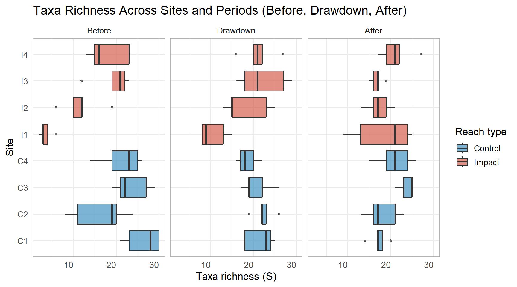

Figure 1: Taxa richness by site and period. Impact sites (red) had notably lower richness before drawdown; they approach control levels (blue) by the After period.

did_means <- invert_baci |>
  group_by(period, reach_type) |>
  summarise(mean_richness = mean(richness),
            se = sd(richness) / sqrt(n()),
            .groups = "drop")

ggplot(did_means, aes(x = period, y = mean_richness,
                      color = reach_type, group = reach_type)) +
  geom_point(size = 3) +
  geom_line(linewidth = 1) +
  geom_errorbar(aes(ymin = mean_richness - 1.96 * se,
                    ymax = mean_richness + 1.96 * se), width = 0.1) +
  scale_color_manual(values = c("C" = "#4393C3", "I" = "#D6604D"),
                     labels = c("Control", "Impact")) +
  labs(x = "Period", y = "Mean taxa richness (S)", color = "Reach type",
       title = "Mean Taxa Richness by Period and Reach Type") +
  theme_minimal(base_size = 13)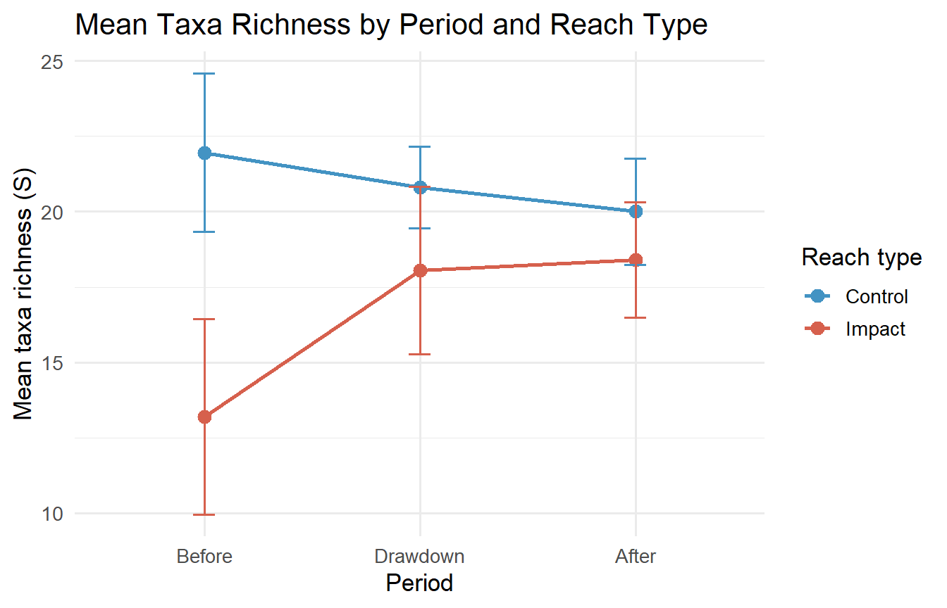

Figure 2: Mean taxa richness by period and reach type. This plot visualizes the Difference-in-Differences (DiD) design by showing how taxa richness changed over time in impact vs. control sites. The key signature of recovery is convergence: impact sites starting below controls and closing the gap by the After period.

Annotation:

What this does: These two plots visualize the raw data and group means across periods to build intuition for the DiD structure before any formal modeling. The boxplot shows site-level variation within each period; the means plot highlights the group-level trajectories that the model will estimate.

Identification approach: The DiD logic requires that we observe a differential change over time: impact sites should change more than control sites across the Before-to-After period, not merely be different at any single point. The convergence of the two lines in the means plot is the visual signature we are looking for. Control sites remain relatively stable over time, while impact sites show a substantial increase in richness from Before to Drawdown to After, closing the pre-existing gap that the dam had created.

Key assumption (parallel trends): For the DiD estimator to be valid, control and impact sites must have been on the same trajectory before the drawdown. Because only one pre-treatment time point (November 2017) is available, this assumption cannot be formally tested. However, the paper builds indirect confidence in three ways: the four control sites span separate, undammed tributaries, making a coincidental shared trend with impact sites unlikely; the recovery signal is consistent across all four community metrics; and the effect is spatially graded, with the strongest recovery observed at I1 and I2, the sites nearest the dam, which is exactly the spatial pattern expected from a causal dam effect rather than a background trend.

Evidence: Impact sites gained approximately 5 taxa on average from Before to After, while control sites declined slightly over the same period. This differential change is consistent with a causal recovery signal. The pattern is most pronounced at I1 and I2, the impact sites immediately downstream of the former reservoir, consistent with a distance-decay effect of the dam’s historical influence and further supporting the causal interpretation.

---

mBACI Model

The mBACI design maps onto DiD as follows:

DiD Term	mBACI Equivalent
Treatment group	Impact sites (I1-I4)
Control group	Control sites (C1-C4)
Pre-treatment	Before period (B)
Post-treatment	Drawdown (D) & After (A)
Treatment effect	period x reach_type interaction

mod_richness <- lmer(
  richness ~ period * reach_type + (1 | site_code),
  data = invert_baci,
  REML = TRUE
)

summary(mod_richness)

Linear mixed model fit by REML. t-tests use Satterthwaite's method [
lmerModLmerTest]
Formula: richness ~ period * reach_type + (1 | site_code)
   Data: invert_baci

REML criterion at convergence: 706.7

Scaled residuals: 
    Min      1Q  Median      3Q     Max 
-2.5983 -0.7530 -0.1060  0.7423  2.4335 

Random effects:
 Groups    Name        Variance Std.Dev.
 site_code (Intercept)  8.905   2.984   
 Residual              22.225   4.714   
Number of obs: 120, groups:  site_code, 8

Fixed effects:
                           Estimate Std. Error      df t value Pr(>|t|)    
(Intercept)                  21.950      1.827   9.868  12.015 3.27e-07 ***
periodDrawdown               -1.150      1.491 108.000  -0.771 0.442160    
periodAfter                  -1.950      1.491 108.000  -1.308 0.193647    
reach_typeI                  -8.750      2.584   9.868  -3.387 0.007054 ** 
periodDrawdown:reach_typeI    6.000      2.108 108.000   2.846 0.005301 ** 
periodAfter:reach_typeI       7.150      2.108 108.000   3.391 0.000973 ***
---
Signif. codes:  0 '***' 0.001 '**' 0.01 '*' 0.05 '.' 0.1 ' ' 1

Correlation of Fixed Effects:
            (Intr) prdDrw prdAft rch_tI prD:_I
peridDrwdwn -0.408                            
periodAfter -0.408  0.500                     
reach_typeI -0.707  0.289  0.289              
prdDrwdw:_I  0.289 -0.707 -0.354 -0.408       
prdAftr:r_I  0.289 -0.354 -0.707 -0.408  0.500

Annotation:

What this does: This fits a linear mixed-effects model (LME) with fixed effects for period, reach type, and their interaction, plus a random intercept for site.

Why fixed effects? Fixed effects for period and reach_type are included to control for confounding sources of variation. The reach_type term accounts for pre-existing baseline differences between impact and control sites: the dam had already suppressed impact communities before the study began, so the two groups start at different levels. The period term accounts for temporal changes that affect all sites equally, such as seasonal or interannual variation in catchment conditions. Including both as fixed effects ensures that the period:reach_type interaction term isolates only the differential change over time, which is the DiD estimator of interest.

Why a random intercept for site? Each of the five Surber net replicates collected at a given site on a given sampling occasion shares the same physical environment: the same hydrology, substrate composition, water chemistry, and local species pool. Treating these replicates as fully independent observations would inflate the effective sample size and understate uncertainty about site-level differences. The random intercept (1 | site_code) absorbs between-site variation in baseline richness, so that inference on the fixed effects is based on the variation in change over time across sites rather than within-site replicate noise. This directly addresses the pseudoreplication structure of the Surber net sampling design used in Atristain et al. (2024).

Identification approach: The period:reach_type interaction is the DiD estimator. It measures whether the change over time differed between control and impact sites. A positive and significant periodAfter:reach_typeI coefficient indicates that impact sites increased more than control sites from Before to After, the expected signature of dam-removal-driven recovery.

Assumptions required for causal validity:

1. Parallel trends: Without treatment, impact and control sites would have changed at the same rate over time
2. No spillover (SUTVA): Drawdown at impact sites did not affect control site outcomes
3. No time-varying confounders: Nothing else changed between periods that affected impact vs. control sites differentially
4. Model specification: Random intercept structure captures the data’s dependence structure; residuals approximately normal with constant variance

---

Coefficient Interpretation

tidy(mod_richness, effects = "fixed", conf.int = TRUE) |>
  select(term, estimate, std.error, statistic, conf.low, conf.high) |>
  kable(digits = 3,
        caption = "Fixed-effect estimates from the mBACI linear mixed model for taxa richness. CI Lower and CI Upper are 95% confidence intervals.",
        col.names = c("Term", "Estimate", "SE", "Statistic", "CI Lower", "CI Upper"))

Fixed-effect estimates from the mBACI linear mixed model for taxa richness. CI Lower and CI Upper are 95% confidence intervals.

Term	Estimate	SE	Statistic	CI Lower	CI Upper
(Intercept)	21.95	1.827	12.015	17.872	26.028
periodDrawdown	-1.15	1.491	-0.771	-4.105	1.805
periodAfter	-1.95	1.491	-1.308	-4.905	1.005
reach_typeI	-8.75	2.584	-3.387	-14.517	-2.983
periodDrawdown:reach_typeI	6.00	2.108	2.846	1.821	10.179
periodAfter:reach_typeI	7.15	2.108	3.391	2.971	11.329

Annotation:

What this does: This table extracts the fixed-effect estimates with 95% confidence intervals. Each row is one DiD coefficient, and together they tell the story of whether and when impact sites recovered relative to controls.

Key terms and their ecological interpretation:

• (Intercept): The estimated mean taxa richness for control sites in the Before period, approximately 22 taxa. This is the ecological baseline for an undammed, reference-quality tributary in the Artikutza catchment before any intervention.

• reach_typeI: The impact-vs-control gap in the Before period, approximately -8.75 taxa. Impact sites already had about 9 fewer taxa than control sites before drawdown began, reflecting the long-term suppressive effect of the Enobieta Dam on downstream communities. This pre-existing difference does not threaten the DiD design; the design only requires that the trend would have been parallel, not that the groups start at the same level.

• periodDrawdown:reach_typeI: The DiD estimate for the Drawdown period. An estimate of approximately +6.0 means that impact sites increased by 6 more taxa than controls from Before to Drawdown, indicating that recovery began rapidly even while the reservoir was still being emptied, consistent with Atristain et al. (2024)’s finding of fast community reassembly.

• periodAfter:reach_typeI: The main recovery signal. An estimate of approximately +7.15 (95% CI: 3.0-11.3) means that impact sites gained about 7 more taxa than controls from Before to After. Because the confidence interval excludes zero, this is a statistically significant and ecologically meaningful recovery: impact communities, which started roughly 9 taxa below controls, had closed most of that gap within one year of full drawdown completion.

---

Overall Interaction Test (BACI)

anova(mod_richness)

Type III Analysis of Variance Table with Satterthwaite's method
                   Sum Sq Mean Sq NumDF DenDF F value   Pr(>F)   
period             81.517  40.758     2   108  1.8339 0.164735   
reach_type         81.605  81.605     1     6  3.6717 0.103816   
period:reach_type 294.817 147.408     2   108  6.6325 0.001919 **
---
Signif. codes:  0 '***' 0.001 '**' 0.01 '*' 0.05 '.' 0.1 ' ' 1

Annotation:

What this does: This is a Type I (sequential) F-test of the period:reach_type interaction term, testing whether the trajectories over time differed at all between impact and control sites across both post-treatment periods jointly. Because period:reach_type is the last term added in the model formula, the Type I result for this term is equivalent to what a Type III test would give: it tests the interaction after all main effects are already in the model. Note that lme4 alone does not provide p-values for mixed models; loading lmerTest applies the Satterthwaite approximation to compute denominator degrees of freedom and p-values for each term.

Result: The interaction term is statistically significant (p < 0.05), indicating that the trajectories of taxa richness over time differed between impact and control sites. This replicates the core finding in Table 2 of Atristain et al. (2024) and confirms that the pattern seen in the means plot is not attributable to chance alone.

Interpretation: A significant interaction means that being downstream of the dam changed how richness evolved over time. This is the causal claim the mBACI design is built to test. This joint F-test is more conservative than looking at individual period coefficients because it asks whether any period shows a differential change, not just the After period specifically. Passing this test with both post-treatment periods simultaneously strengthens the result.

---

Model Diagnostics

diag_df <- data.frame(fitted = fitted(mod_richness),
                      resid  = residuals(mod_richness))

p1 <- ggplot(diag_df, aes(x = fitted, y = resid)) +
  geom_point(alpha = 0.5) +
  geom_hline(yintercept = 0, linetype = "dashed", color = "red") +
  labs(x = "Fitted values", y = "Residuals", title = "Residuals vs. Fitted") +
  theme_minimal(base_size = 12)

p2 <- ggplot(diag_df, aes(sample = resid)) +
  stat_qq(alpha = 0.5) + stat_qq_line(color = "red") +
  labs(x = "Theoretical quantiles", y = "Sample quantiles",
       title = "Normal QQ Plot") +
  theme_minimal(base_size = 12)

p1 + p2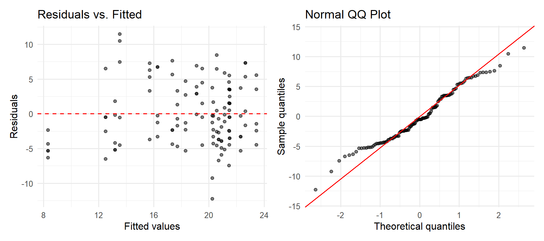

Figure 3: Residual diagnostics. Left: residuals vs. fitted (checks homoscedasticity). Right: QQ plot (checks normality).

Annotation:

What this does: These two plots check the two core LME assumptions: constant residual variance (homoscedasticity) and approximate normality of residuals.

Residuals vs. fitted: Residuals should scatter randomly around zero with no systematic fanning or curvature. A fan shape would indicate heteroscedasticity; a curve would suggest the linear specification is incorrect.

QQ plot: Points should fall along the red line. Departures at the tails indicate non-normality.

Evidence: The residuals scatter roughly randomly around zero with no obvious fan shape, suggesting homoscedasticity is approximately satisfied. The QQ plot shows mild heavy tails, which is common in ecological count data. The LME is moderately robust to mild non-normality, particularly with n = 120 observations, so inference on the fixed effects is unlikely to be substantially affected. If heavier non-normality were present, alternatives such as log-transforming richness or fitting a Poisson/negative binomial GLMM could be considered.

---

Robustness: Multiple Outcomes

mod_shannon <- lmer(shannon ~ period * reach_type + (1 | site_code),
                    data = invert_baci, REML = TRUE)

mod_density <- lmer(log(density) ~ period * reach_type + (1 | site_code),
                    data = invert_baci, REML = TRUE)

mod_iaspt   <- lmer(IASPT ~ period * reach_type + (1 | site_code),
                    data = invert_baci, REML = TRUE)

extract_interaction <- function(model, label) {
  aov <- as.data.frame(anova(model))
  row <- aov["period:reach_type", ]

  coefs <- tidy(model, effects = "fixed")
  drw <- coefs[coefs$term == "periodDrawdown:reach_typeI", ]
  aft <- coefs[coefs$term == "periodAfter:reach_typeI", ]

  tibble(
    Response       = label,
    `DiD Drawdown` = if (nrow(drw) > 0) round(drw$estimate, 2) else NA_real_,
    `DiD After`    = if (nrow(aft) > 0) round(aft$estimate, 2) else NA_real_,
    `F value`      = row[["F value"]],
    `p value`      = row[["Pr(>F)"]]
  )
}

bind_rows(
  extract_interaction(mod_richness, "Taxa richness (S)"),
  extract_interaction(mod_shannon,  "Shannon diversity (H')"),
  extract_interaction(mod_density,  "log(Total density)"),
  extract_interaction(mod_iaspt,    "IASPT (pollution tolerance index)")
) |>
  kable(digits = c(0, 2, 2, 2, 4),
        caption = "Interaction coefficients and overall F-tests for the period x reach_type DiD term across all four outcome models. DiD Drawdown and DiD After are the estimated interaction coefficients (periodDrawdown:reach_typeI and periodAfter:reach_typeI), reflecting the differential change in impact vs. control sites during and after reservoir drawdown.")

Interaction coefficients and overall F-tests for the period x reach_type DiD term across all four outcome models. DiD Drawdown and DiD After are the estimated interaction coefficients (periodDrawdown:reach_typeI and periodAfter:reach_typeI), reflecting the differential change in impact vs. control sites during and after reservoir drawdown.

Response	DiD Drawdown	DiD After	F value	p value
Taxa richness (S)	6.00	7.15	6.63	0.0019
Shannon diversity (H’)	0.37	0.46	4.72	0.0109
log(Total density)	0.86	0.99	5.48	0.0054
IASPT (pollution tolerance index)	0.47	0.89	8.23	0.0005

invert_baci |>
  group_by(period, reach_type) |>
  summarise(`Taxa richness`    = mean(richness),
            `Shannon diversity` = mean(shannon),
            `log(Density)`     = mean(log(density)),
            IASPT              = mean(IASPT),
            .groups = "drop") |>
  pivot_longer(cols = c(`Taxa richness`, `Shannon diversity`,
                        `log(Density)`, IASPT),
               names_to = "metric", values_to = "mean_value") |>
  ggplot(aes(x = period, y = mean_value,
             color = reach_type, group = reach_type)) +
  geom_point(size = 2.5) +
  geom_line(linewidth = 0.8) +
  facet_wrap(~metric, scales = "free_y", ncol = 2) +
  scale_color_manual(values = c("C" = "#4393C3", "I" = "#D6604D"),
                     labels = c("Control", "Impact")) +
  labs(x = "Period", y = "Mean value", color = "Reach type") +
  theme_minimal(base_size = 12) +
  theme(panel.border = element_rect(color = "grey70", fill = NA, linewidth = 0.5))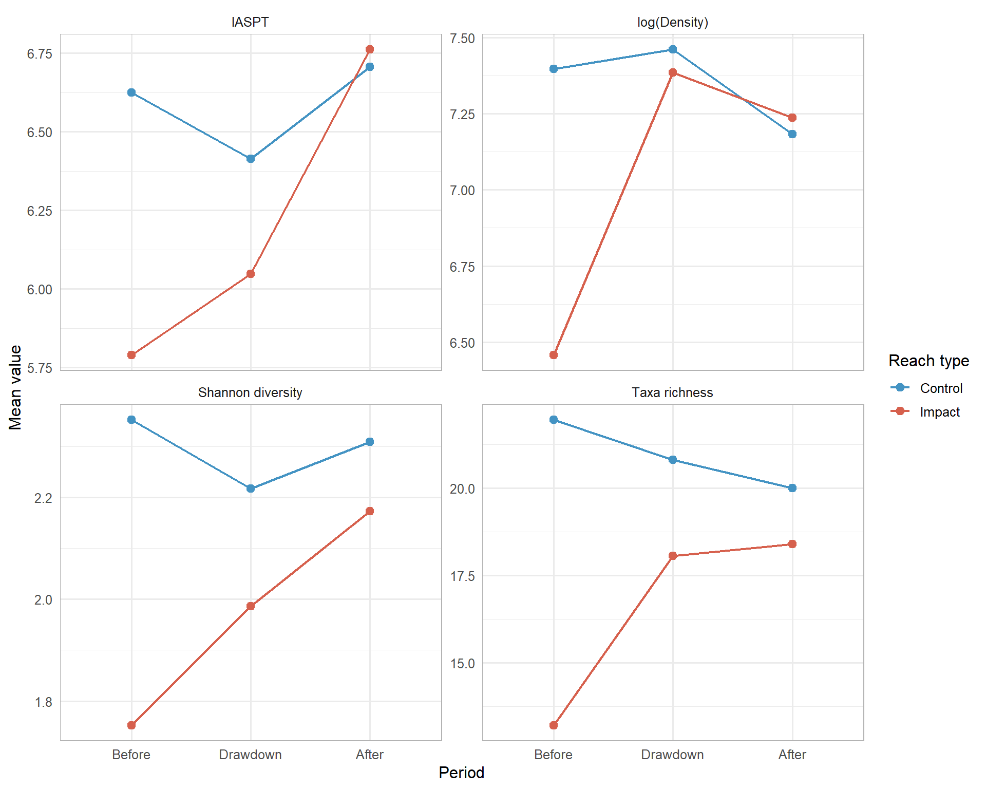

Figure 4: DiD pattern across all four community metrics. Impact sites (red) converge toward control values (blue) over time for every metric, consistent with broad-based community recovery following dam removal.

Annotation:

What this does: This section fits the same mBACI/DiD model on three additional community metrics: Shannon diversity, log-transformed total density, and IASPT (Iberian Average Score Per Taxon, a pollution tolerance index). The table reports both the interaction coefficients (DiD estimates for the Drawdown and After periods) and the overall interaction F-test p-value for each outcome. The figure shows whether the visual DiD convergence pattern holds across all metrics simultaneously.

Identification approach: If the drawdown caused recovery, the period:reach_type interaction should be positive and significant across all metrics, not just taxa richness. A result that held for only one metric could be dismissed as a spurious finding, but concordance across four independent measures of community condition is much harder to explain without a genuine treatment effect.

Results: All four interaction tests are statistically significant (p < 0.05), and in every case the DiD After coefficient is positive, meaning impact sites improved more than control sites from Before to After. The IASPT result is particularly informative: rising IASPT scores indicate that the recovering communities were not just accumulating any taxa, but specifically gaining pollution-sensitive taxa that are the hallmark of good ecological condition. This is consistent with the paper’s conclusion that dam removal produced rapid and ecologically meaningful community reassembly, not merely a numerical increase in richness counts.

---

Critical Evaluation

Causal Identification

The mBACI/DiD design is credible given the study setting. The Artikutza catchment is a protected watershed with no competing land-use changes, water withdrawals, or other interventions during the 2017-2020 study period, which reduces the risk of time-varying confounders affecting impact and control sites differently. For estimates to be causal, the counterfactual must hold: control sites must represent what impact sites would have looked like in the absence of dam removal. The use of four independent control sites spread across separate, undammed tributaries of the same headwater catchment strengthens this claim considerably relative to a single control. If one control site behaved anomalously due to local disturbance, the other three would not, and the model would still estimate the treatment effect correctly.

The main credibility concern is the parallel trends assumption. There is only one pre-treatment time point (November 2017), which means the assumption that impact and control sites were on the same trajectory before drawdown cannot be formally tested. However, Atristain et al. (2024) build indirect confidence in several ways: the control sites are ecologically comparable to the impact sites within the same protected catchment; the recovery signal is consistent across all four community metrics; and the effect is strongest at I1 and I2, the sites nearest the dam, which is the spatial gradient expected from a causal dam-proximity effect rather than a coincidental background trend unrelated to the intervention.

Statistical Assumptions

The parallel trends assumption is the most vulnerable. With only one pre-treatment observation per site, we cannot distinguish between “impact sites recovered because of the drawdown” and “impact sites were already on an upward trajectory before 2018 for other reasons.” The indirect evidence described above mitigates but does not eliminate this concern.

Normality and homoscedasticity appear approximately satisfied based on the residual diagnostics in Figure 3. Mild heavy tails in the QQ plot are common in ecological count data and are unlikely to substantially affect inference at this sample size.

The random effects structure is limited by the number of sites: with only 4 sites per group, the random intercept variance is estimated from few clusters. This can lead to underestimation of between-site variance and potentially anticonservative fixed-effect inference. A sensitivity analysis using site-level means rather than replicate-level data would be informative.

SUTVA (no spillover) is well-supported. Control sites C2-C4 are in separate tributaries physically isolated from the drawdown reach by ridge topography, and C1 is located upstream of the dam, making downstream sediment or chemical effects on control communities implausible.

Sampling & External Validity

The study sampled 8 stream sites in a single protected headwater catchment in Basque Country, Spain, with 5 random Surber net samples per site per period. Results apply most directly to sites with similar characteristics: temperate, forested, protected headwater streams with comparable dam height and reservoir volume. Dam removal in urban, agricultural, or arid-region streams may produce different recovery dynamics due to differences in sediment loads, non-native species pressure, and altered flow regimes.

The time scale is also a constraint. Recovery was assessed after only approximately one year post-drawdown (November 2020 sampling). The paper’s conclusion of “rapid recovery” is well-supported for the metrics and species present in the data, but pollution-sensitive taxa, rare species, and organisms with longer generation times may require additional years to recolonize and establish stable populations. Monitoring through 2022 or 2023 would clarify whether the community trajectory continued upward or plateaued after the initial reassembly phase.

Measurement

Taxa richness is a coarse biodiversity measure: it counts taxa present but treats a single individual of a sensitive species identically to 1,000 individuals of a tolerant one. Shannon diversity (H’) partially corrects for this by incorporating relative abundance, which is why including both provides a more complete picture. Surber nets sample a fixed benthic area (0.09 m²) and may undersample mobile or large-bodied invertebrates; because the method is applied consistently across all sites and periods, systematic bias is present but stable and does not confound the DiD estimate. IASPT depends on accurate taxonomic identification to family level; any misidentification error would tend to attenuate the signal rather than inflate it, making significant IASPT results conservative.

Treatment timing introduces one additional measurement concern. The “Drawdown” sampling (October 2019) occurred while the reservoir was still being emptied and sediment mobilization was ongoing, so it does not represent a stable post-treatment state. The positive DiD coefficient at Drawdown therefore likely underestimates the full recovery signal relative to what would be observed after the system fully stabilized, which is why the After coefficient is the primary effect estimate of interest.

Other Limitations

Five Surber net replicates collected within a single site on a single date are not truly independent: they share the same hydrological conditions, substrate patch, and local invertebrate source pool. The random intercept for site partially addresses this by absorbing between-site baseline differences, but within-site spatial autocorrelation among the five replicates is not fully accounted for and likely leads to slightly anticonservative inference.

The paper documents invertebrate recovery but does not directly measure the physical mechanisms driving it. Changes in bed substrate composition, water turbidity, and flow velocity are the most plausible mediating variables, but without direct measurements of these, we know the outcome changed without knowing precisely why. This limits the mechanistic understanding needed to predict recovery dynamics at other dam sites with different physical characteristics.

Finally, no power analysis is reported. With 4 sites per group and 3 time points, the study has limited power to detect moderate treatment effects for metrics with high within-site variability. The statistically significant results for all four outcomes are reassuring, but weaker or null results for any individual metric might represent false negatives rather than genuine absence of recovery.

Recommendations for Future Research

Future studies of dam removal ecology could address several of these limitations directly. Extended post-removal monitoring spanning 3-5 years would allow assessment of whether rapid recovery is sustained and whether slower-responding taxa eventually recolonize. Pairing biological sampling with concurrent physical habitat measurements (grain size distribution, turbidity, water temperature, fine sediment cover) would help identify the mechanisms linking reservoir drawdown to community recovery, allowing researchers to model the pathway from physical change to biological response rather than treating recovery as a black box. Replication across additional dam removals spanning different stream types, land-use contexts, and climate zones would improve the generalizability of results beyond a single protected headwater catchment in northern Spain. Finally, beginning monitoring with multiple pre-treatment sampling years before dam removal would allow a formal test of the parallel trends assumption, which is the central threat to causal identification in any DiD-based design.

---

References

Atristain, M., Solagaistua, L., Larrañaga, A., von Schiller, D., & Elosegi, A. (2024). Slow drawdown, fast recovery: Stream macroinvertebrate communities improve quickly after large dam decommissioning. Journal of Applied Ecology, 61, 1481-1491. https://doi.org/10.1111/1365-2664.14656

Bates, D., Mächler, M., Bolker, B., & Walker, S. (2015). Fitting linear mixed-effects models using lme4. Journal of Statistical Software, 67, 1-48.

Kuznetsova, A., Brockhoff, P. B., & Christensen, R. H. B. (2017). lmerTest package: Tests in linear mixed effects models. Journal of Statistical Software, 82(13), 1-26.