
Code
# Import required libraries for geospatial analysis and visualization
import xarray as xr
import rioxarray as rio
import geopandas as gpd
import pandas as pd
import numpy as np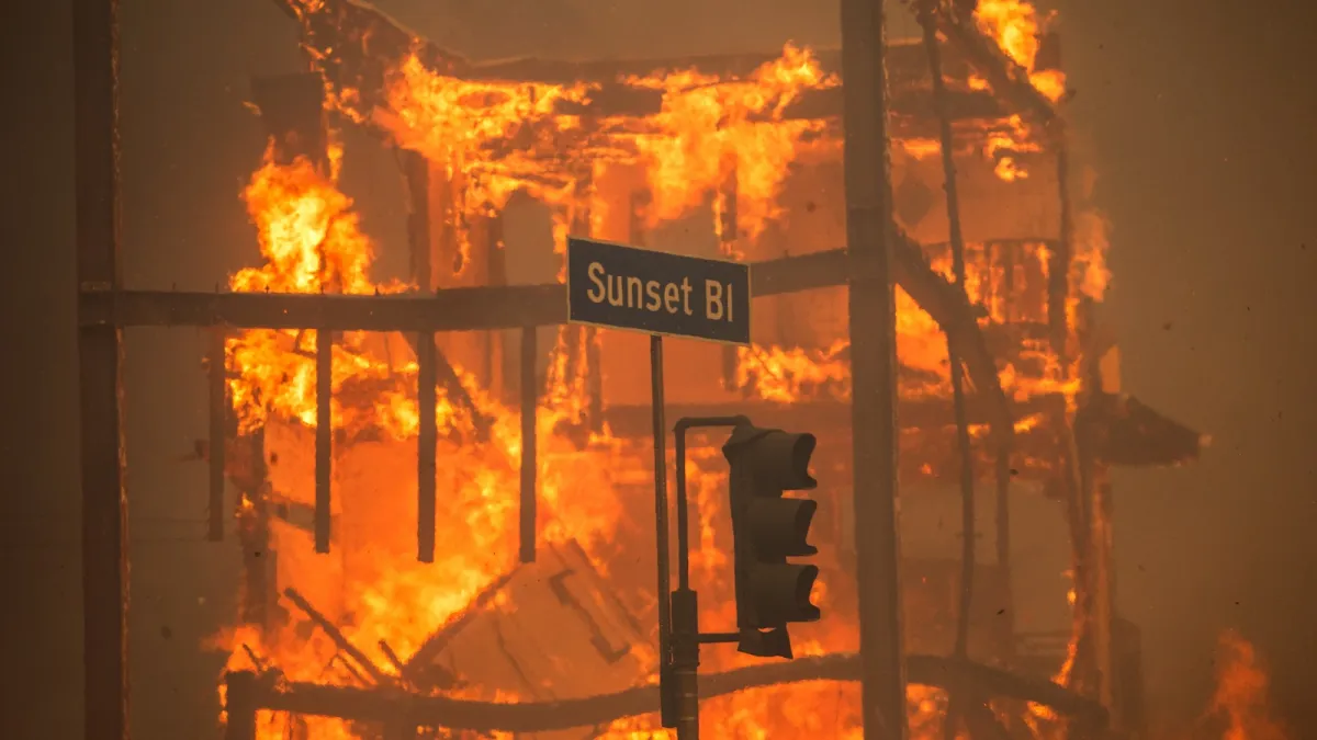
import matplotlib.pyplot as pltIn January 2025, the Eaton and Palisades fires swept through Los Angeles County, leaving lasting impacts on both the landscape and the communities within their paths. The Palisades Fire, which started on January 7, became one of the most destructive wildfires in California history, burning through the scenic Pacific Palisades neighborhood and nearby communities. Meanwhile, the Eaton Fire ignited in the foothills near Altadena and Pasadena, threatening densely populated areas and critical infrastructure.
Understanding wildfire impacts requires more than just mapping burned areas-it requires examining both the physical changes to the landscape and the social dimensions of who is affected. This analysis combines remote sensing techniques with environmental justice data to provide a comprehensive view of these devastating fires.
Repository: https://github.com/rellimylime/eaton-palisades-fires-analysis For complete analysis notebooks with additional data exploration and detailed outputs, visit the GitHub repository.
This analysis demonstrates several key Python-based geospatial analysis techniques:
xarray and rioxarray to process Landsat 8 SWIR/NIR/Red bands for burn scar identificationgeopandas combining satellite raster imagery with vector fire perimeter and census tract datario.write_crs() and to_crs() to ensure spatial alignment across different data sourcesgpd.sjoin()) and clipping to examine racial demographics in fire-affected areasThis dataset contains atmospherically corrected surface reflectance data from the Landsat 8 satellite, captured on February 23, 2025 (Microsoft Planetary Computer 2025). The imagery includes five spectral bands (red, green, blue, near-infrared, and shortwave infrared) clipped to the area surrounding the Eaton and Palisades fire perimeters. The data was retrieved from the Microsoft Planetary Computer STAC catalog in NetCDF format.
These shapefiles delineate the official fire perimeters for the Eaton and Palisades fires as of January 21, 2025 (ArcGIS Hub 2025). The vector data includes boundary geometries and attribute information for each fire.
The CDC/ATSDR Environmental Justice Index (Centers for Disease Control and Prevention and Agency for Toxic Substances and Disease Registry 2024) provides census tract-level demographic and socioeconomic data. This analysis uses the 2024 California EJI dataset to examine the racial composition of fire-affected communities through minority population percentile rankings.
# Import required libraries for geospatial analysis and visualization
import xarray as xr
import rioxarray as rio
import geopandas as gpd
import pandas as pd
import numpy as np
import matplotlib.pyplot as pltFire perimeters provide the spatial boundaries for our analysis, allowing us to focus on the areas most affected by the fires.
# Load fire perimeter shapefiles
eaton = gpd.read_file('data/Eaton_Perimeter_20250121.shp')
palisades = gpd.read_file('data/Palisades_Perimeter_20250121.shp')

# Create summary table for data exploration
summary_data = {
    'Dataset': ['Eaton Fire', 'Palisades Fire'],
    'Features': [len(eaton), len(palisades)],
    'Columns': [len(eaton.columns), len(palisades.columns)],
    'Geometry Type': [eaton.geometry.type.unique()[0], palisades.geometry.type.unique()[0]]
}

summary_df = pd.DataFrame(summary_data)

# Display as formatted table
summary_df
Both datasets contain polygon geometries representing the fire boundaries, along with area and perimeter measurements.
# Create CRS information table
crs_data = {
    'Dataset': ['Eaton Fire', 'Palisades Fire'],
    'CRS Code': [eaton.crs.to_authority()[1] if eaton.crs.to_authority() else 'N/A',
                 palisades.crs.to_authority()[1] if palisades.crs.to_authority() else 'N/A'],
    'Projection Type': ['Geographic' if eaton.crs.is_geographic else 'Projected',
                       'Geographic' if palisades.crs.is_geographic else 'Projected']
}

crs_df = pd.DataFrame(crs_data)

# Display as formatted table
crs_df
Both datasets use EPSG:3857 (Web Mercator), a projected coordinate system suitable for web mapping applications.
The Landsat 8 scene contains multiple spectral bands that capture different wavelengths of reflected light. Each band provides unique information about surface features.
# Import Landsat data
landsat = xr.open_dataset('data/landsat8-2025-02-23-palisades-eaton.nc')

# Create Landsat dataset summary table
landsat_summary = {
    'Property': ['Dimensions', 'Height (y)', 'Width (x)', 'Coordinates', 'Data Variables'],
    'Value': [
        f"{len(landsat.dims)}D",
        f"{landsat.dims['y']} pixels",
        f"{landsat.dims['x']} pixels",
        ', '.join(list(landsat.coords)),
        ', '.join([v for v in landsat.data_vars if v != 'spatial_ref'])
    ]
}

landsat_df = pd.DataFrame(landsat_summary)

# Display as formatted table
landsat_df
The dataset spans 1418 × 2742 pixels and contains five spectral bands: red, green, blue, nir08, swir22.
Before we can perform spatial operations, we need to verify and restore the coordinate reference system (CRS) information.
# Recover the geospatial information from spatial_ref
landsat = landsat.rio.write_crs(landsat.spatial_ref.crs_wkt)
The dataset’s CRS is restored from the
spatial_refmetadata variable, setting it to EPSG:32611 (WGS 84 / UTM zone 11N), which is appropriate for the Los Angeles area.
# Check for NaN values in each band
bands = ['red', 'green', 'blue', 'nir08', 'swir22']
nan_status = []

for band in bands:
    has_nan = np.isnan(landsat[band]).any().values
    nan_count = np.isnan(landsat[band]).sum().values
    nan_status.append({
        'Band': band.upper(),
        'Contains NaN': 'Yes' if has_nan else 'No',
        'NaN Count': int(nan_count)
    })

nan_df = pd.DataFrame(nan_status)

# Display as formatted table
nan_df# Fill NaN values with 0
landsat = landsat.fillna(0)All five spectral bands contain NaN values at the edges of the scene or in clouded areas. These are filled with zero to prevent visualization errors.
Before creating specialized visualizations, we can verify our data by creating a true color image using the red, green, and blue bands-similar to how a standard camera would capture the scene.
# Create true color composite with robust scaling
# Coarsen by factor of 4 to reduce memory usage
landsat_viz = landsat[['red', 'green', 'blue']].coarsen(x=4, y=4, boundary='trim').mean()
landsat_viz.to_array().plot.imshow(robust=True)
plt.title('True Color Image - Landsat 8')
plt.tight_layout()
The
robust=Trueparameter clips extreme outlier values to improve visualization, preventing a few bright pixels from washing out the entire image.
False color composites use non-visible wavelengths to reveal features invisible to the human eye. By assigning shortwave infrared (SWIR) to red, near-infrared (NIR) to green, and red to blue, we create an image where healthy vegetation appears bright green and burned areas show distinct reddish-brown tones.
# Create false color composite (SWIR/NIR/Red)
# Coarsen by factor of 4 to reduce memory usage
landsat_false = landsat[['swir22', 'nir08', 'red']].coarsen(x=4, y=4, boundary='trim').mean()
landsat_false.to_array().plot.imshow(robust=True)
plt.title('False Color Composite (SWIR/NIR/Red)')
plt.tight_layout()
Why this band combination?
- Healthy vegetation has high NIR reflectance and low SWIR reflectance → appears bright green
- Burned areas have low NIR reflectance and moderate SWIR reflectance → appears reddish-brown
- Urban areas show moderate reflectance across bands → appears in neutral tones
To provide geographic context, we overlay the fire perimeters onto our false color image. This requires reprojecting the vector data to match the raster’s coordinate system (EPSG:32611 - UTM Zone 11N).
# Reproject fire perimeters to match Landsat CRS
eaton = eaton.to_crs(landsat.rio.crs)
palisades = palisades.to_crs(landsat.rio.crs)

# Create comprehensive map
fig, ax = plt.subplots(figsize = (12, 12))

# Plot false color composite (downsampled for memory efficiency)
landsat_map = landsat[['swir22', 'nir08', 'red']].coarsen(x=4, y=4, boundary='trim').mean()
landsat_map.to_array().plot.imshow(
    ax = ax,
    robust = True,
    add_colorbar = False
)

# Overlay fire perimeters
eaton.boundary.plot(ax = ax, edgecolor = 'yellow', linewidth = 2, label = 'Eaton Fire')
palisades.boundary.plot(ax = ax, edgecolor = 'red', linewidth = 2, label = 'Palisades Fire')

# Add labels and formatting
plt.title('Eaton and Palisades Fires - False Color Analysis',
          fontsize = 20, fontweight = 'bold', pad = 20)
plt.legend(loc = 'upper right', fontsize = 14)
ax.set_xlabel('Easting (meters)', fontsize = 14)
ax.set_ylabel('Northing (meters)', fontsize = 14)

# Add fire name annotations
ax.text(eaton.geometry.centroid.x.values[0],
        eaton.geometry.centroid.y.values[0] - 2700,
        'Eaton Fire',
        color = 'black', fontsize = 14, fontweight = 'bold',
        bbox = dict(boxstyle = 'round', facecolor = 'white', alpha = 0.7))

ax.text(palisades.geometry.centroid.x.values[0] - 22000,
        palisades.geometry.centroid.y.values[0] + 8000,
        'Palisades Fire',
        color = 'black', fontsize = 14, fontweight = 'bold',
        bbox = dict(boxstyle = 'round', facecolor = 'white', alpha = 0.7))

plt.tight_layout()
plt.show()This false color composite displays the Eaton and Palisades fire areas captured by Landsat 8 on February 23, 2025. The image uses shortwave infrared (SWIR), near-infrared (NIR), and red bands to highlight burn scars and vegetation health.
Key features:
- Bright green areas = Healthy vegetation (high NIR reflectance)
- Reddish-brown areas = Burned areas and bare soil (low NIR, moderate SWIR)
- Urban/developed areas = Neutral tones (moderate reflectance across bands)
The fire perimeters are overlaid in yellow (Eaton Fire) and red (Palisades Fire) to delineate the official burn boundaries. This false color combination is particularly effective for assessing fire severity and monitoring landscape recovery, as the spectral signatures of healthy vs. burned vegetation are distinctly different in the infrared wavelengths.
Wildfires don’t impact all communities equally. This analysis examines the racial composition of census tracts affected by the fires to understand environmental justice implications.
The EJI dataset contains census tract-level data for all of California with 174 columns including demographic, environmental, and health vulnerability indicators. Both the EJI data and fire perimeters use EPSG:3857 (Web Mercator) coordinate reference system.
To understand which communities were directly impacted by the fires, we use spatial intersection operations to identify census tracts that overlap with the fire perimeters. We then clip these tracts to the exact fire boundaries, ensuring our analysis focuses only on the areas that experienced direct fire impacts rather than nearby unaffected regions.
The Environmental Justice Index includes percentile rankings for demographic characteristics. Here we examine EPL_MINRTY, which represents the percentile rank of minority population (persons of color)-a measure of racial and ethnic composition relative to other California communities.
fig, (ax1, ax2) = plt.subplots(1, 2, figsize = (18, 9))

# Define variable to analyze
eji_variable = 'EPL_MINRTY'

# Scale values to 0-100 for proper percentile display
eji_clip_palisades_scaled = eji_clip_palisades.copy()
eji_clip_eaton_scaled = eji_clip_eaton.copy()

# Multiply by 100 to convert to percentile
eji_clip_palisades_scaled[eji_variable] = eji_clip_palisades[eji_variable] * 100
eji_clip_eaton_scaled[eji_variable] = eji_clip_eaton[eji_variable] * 100

# Define common scale for comparison (0-100)
vmin = 0
vmax = 100

# Palisades Fire area
eji_clip_palisades_scaled.plot(
    column = eji_variable,
    vmin = vmin, vmax = vmax,
    cmap = 'YlOrRd',
    legend = False,
    ax = ax1,
    edgecolor = 'black',
    linewidth = 0.5
)
ax1.set_title('Minority Population\nPalisades Fire Area', fontsize = 20)
ax1.axis('off')

# Eaton Fire area
eji_clip_eaton_scaled.plot(
    column = eji_variable,
    vmin = vmin, vmax = vmax,
    cmap = 'YlOrRd',
    legend = False,
    ax = ax2,
    edgecolor = 'black',
    linewidth = 0.5
)
ax2.set_title('Minority Population\nEaton Fire Area', fontsize = 20)
ax2.axis('off')

# Overall title
fig.suptitle('Percentile Rank of Minority Population in Fire-Affected Areas',
fontsize = 25, y = 0.98)

# Shared colorbar
sm = plt.cm.ScalarMappable(
    cmap = 'YlOrRd',
    norm = plt.Normalize(vmin = vmin, vmax = vmax)
)
cbar_ax = fig.add_axes([0.25, 0.12, 0.5, 0.03])
cbar = fig.colorbar(sm, cax = cbar_ax, orientation = 'horizontal')
cbar.set_label('Percentile Rank (0-100)', fontsize = 18)
cbar.ax.tick_params(labelsize=16)

plt.tight_layout()
plt.show()The demographic analysis reveals stark differences in the racial composition of communities affected by the two fires. The maps show percentile rankings of minority population, where higher values indicate greater representation of people of color relative to other California census tracts.
Palisades Fire Area: Predominantly low percentile rankings (0th-30th percentiles, pale yellow). The fire primarily impacted areas with very low proportions of minority residents-a predominantly white, affluent coastal community.
Eaton Fire Area: Dramatically high percentile rankings (70th-100th percentiles, dark red). Nearly the entire burn area shows the highest minority population concentrations in the state. The Eaton fire overwhelmingly affected communities of color, particularly in Altadena.
Implications for Recovery:
Research on disaster recovery consistently shows that communities of color face systemic barriers including reduced insurance coverage, limited financial reserves, and difficulties navigating aid bureaucracies. Identifying the demographic composition of affected areas is a critical first step for targeting recovery resources and monitoring for equitable outcomes. Future analysis should examine differential resource allocation, damage assessments, and recovery timelines to assess whether these fires followed historical patterns of inequitable disaster response.
This analysis shows that proximity doesn’t mean equal impact. Though geographically close, the Eaton and Palisades fires had profoundly different social consequences. The Palisades fire affected wealthy, predominantly white neighborhoods. The Eaton fire devastated communities of color already facing systemic barriers to recovery.
The combination of xarray, rioxarray, and geopandas transforms wildfire analysis from purely physical assessment to social justice documentation. Satellite data shows where fires burned; census data reveals whose communities bore the burden. As climate change intensifies California wildfires, these integrated approaches become essential for equity-centered disaster response and recovery planning that addresses the structural inequalities behind disparate climate impacts.
@online{miller2025,
  author = {Miller, Emily},
  title = {Burn {Scars} and {Unequal} {Burdens}},
  date = {2025-11-29},
  url = {https://rellimylime.github.io/posts/eds220-final/},
  langid = {en}
}